Getting Started with VLOOKUP: A Beginner's Guide

About this edition: This independently rewritten article follows a topic and page address found on the public Formula Explainer blog. It is not an extracted Wayback snapshot.

Understanding the problem

VLOOKUP searches down the first column of a table and retrieves a value from a column to its right. It is useful for matching product codes, staff IDs, and categories when the lookup key occupies the leftmost column.

Before changing a formula, write down what a correct result would look like and which rows, columns, or values should contribute to it. This prevents a quick fix from hiding an unrelated error elsewhere in the workbook.

Start with a concrete formula

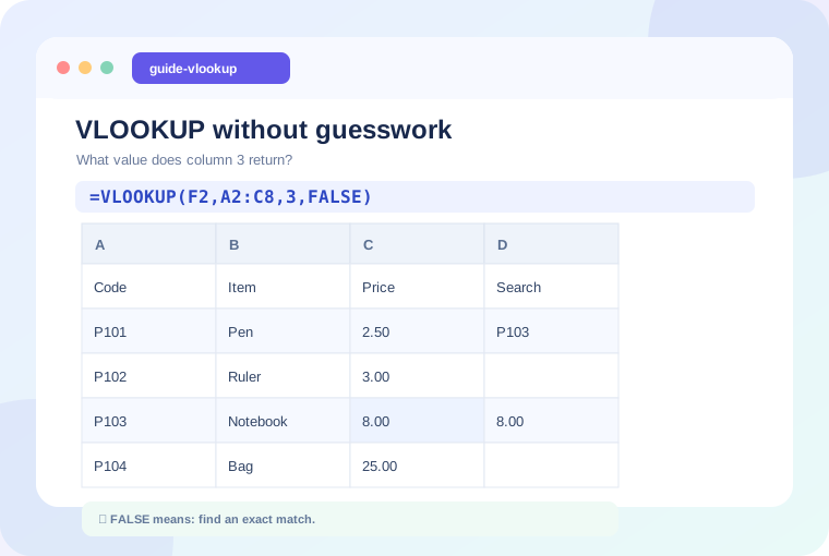
=VLOOKUP(F2,A2:D40,3,FALSE)

In the example, F2 supplies the key, A2:D40 is the table, 3 selects its third column, and FALSE requests an exact match. A common beginner mistake is thinking 3 means the worksheet’s column C rather than the third column inside the selected table.

Read the expression from its inner operations toward the outside, paying attention to references, quoted text, and the conditions that determine which values are included. If your spreadsheet uses semicolon separators, adapt the example to your regional settings.

A practical troubleshooting method

Lock your table range with dollar signs when copying down, ensure identifiers share a consistent data type, and inspect the table’s first column for the key. Avoid approximate matching unless the data is deliberately prepared for it.

1. Duplicate the worksheet or save a new version before experimenting with an important workbook.
2. Compare the expected result with the actual result using a small sample whose answer can be checked by hand.
3. Check numeric and text formats and confirm that each cell reference points to the intended data.
4. Test intermediate expressions separately, then put the full formula together again.
5. Copy the correction into representative rows and check that relative and absolute references behave as expected.

Practice the concept

Make a four-column product table, search for one existing item and one missing item, and observe the behavior. If you need to return values from the left, explore XLOOKUP or INDEX/MATCH.

For best results, test one normal case, one boundary case, and one intentionally invalid case. A formula becomes trustworthy when the expected outcomes are explicit and reproducible.

Common pitfalls to avoid

• Assuming the displayed data type: values may look numeric even when stored as text.
• Hiding a calculation error: use IFERROR only when you have decided how failures should be handled.
• Ignoring worksheet context: a correct expression pointing to the wrong range is still a wrong calculation.
• Skipping version checks: some functions are not supported in older Excel or Sheets versions.

Summary and next step

The reliable approach is to understand each argument, validate the input data, and confirm the intended result with a small experiment. Use a helper column when it makes the logic easier for another person to review. You can also copy the example into the browser-based explainer to explore its structure.